Spatial autocorrelation is a key concept in geographic data analysis. It describes the degree to which the value of a variable at one location is similar to its values at nearby locations. Think of it as measuring the "spatial relationship" between data points.
This principle is widely used in Geographic Information Systems (GIS) to analyze patterns, trends, and relationships in spatial data.
What is Spatial Autocorrelation?
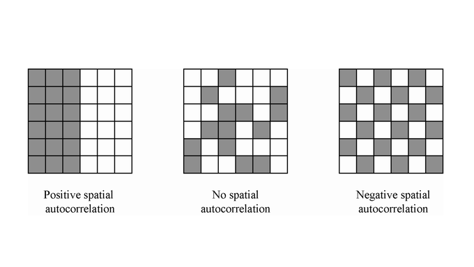
Spatial autocorrelation occurs when geographic data values are not randomly distributed across space. Instead, they exhibit patterns that are either clustered (similar values appear near each other) or dispersed (different values appear near each other).
- Positive Spatial Autocorrelation: Nearby locations have similar values. For example, areas with high property prices tend to be surrounded by other high-priced areas.
- Negative Spatial Autocorrelation: Nearby locations have dissimilar values. An example might be urban areas (high population density) neighboring rural areas (low population density).
- No Spatial Autocorrelation: There is no discernible spatial pattern; the values are randomly distributed.

Why is Spatial Autocorrelation Important?
In spatial analysis, assuming data independence can lead to inaccurate results if spatial autocorrelation exists. Here's why it matters:
-
Pattern Recognition
It helps identify and interpret patterns within geographic data. For instance, detecting clusters of diseases in public health. -
Improved Decision-Making
Planners can use insights about spatial autocorrelation to allocate resources effectively, such as targeting high-crime areas for increased policing. -
Model Accuracy
Recognizing autocorrelation ensures that predictive models account for spatial relationships, leading to better accuracy in forecasts.
Measuring Spatial Autocorrelation
Spatial autocorrelation is quantified using statistical measures. The two most common methods are:
Moran's I
This global indicator measures the degree of spatial autocorrelation across the entire dataset.
- Value range: From -1 to +1.
- A positive value indicates clustering of similar values.
- A negative value indicates dispersion.
- A value near zero implies random distribution.
Geary's C
Similar to Moran’s I but focuses on differences between neighboring data points.
- Value range: From 0 to 2.
- A value of 1 indicates no spatial autocorrelation.
- Values below 1 show positive spatial autocorrelation.
- Values above 1 indicate negative spatial autocorrelation.
Both measures depend on a spatial weights matrix, which defines how the proximity of data points is calculated.
Real-World Applications of Spatial Autocorrelation
1. Urban Planning
Urban planners use spatial autocorrelation to identify housing clusters, traffic congestion zones, or areas lacking amenities.
2. Public Health
It helps in tracking the spread of diseases, understanding environmental health hazards, and identifying healthcare accessibility gaps.
3. Environmental Studies
Spatial autocorrelation aids in studying natural phenomena like climate patterns, vegetation distributions, and pollution sources.
4. Crime Analysis
Law enforcement agencies leverage spatial autocorrelation to detect crime hotspots and deploy resources effectively.
How Spatial Autocorrelation is Used in Atlas
Atlas, a browser-based GIS platform, simplifies spatial analysis, including tasks involving spatial autocorrelation. Here's how it supports such analyses:
-
Interactive Mapping
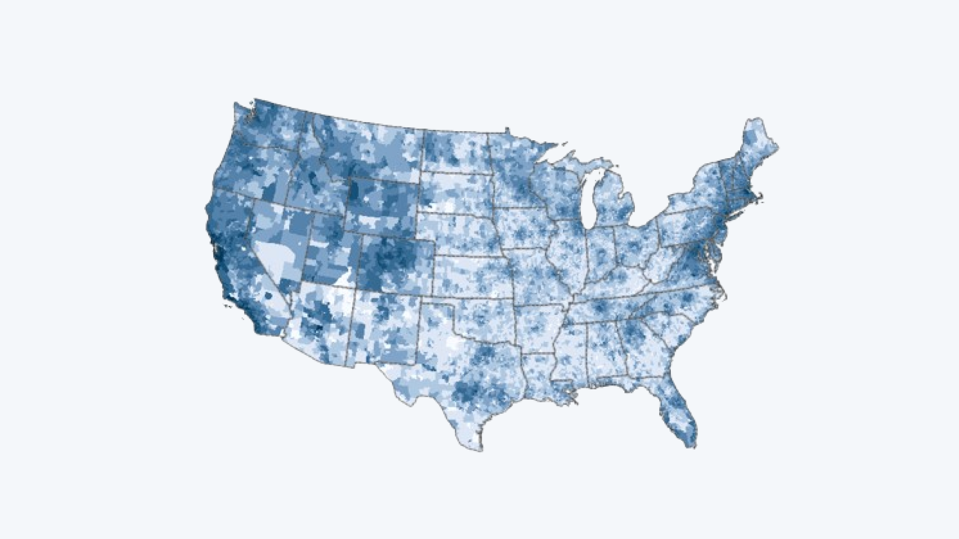
Users can visualize clusters directly on the map. For example, seeing income levels by region. -
Layer Customization
Style map layers to highlight areas of positive or negative spatial autocorrelation. -
Statistical Analysis Tools
Built-in tools can generate heatmaps to identify hotspots.
Challenges in Spatial Autocorrelation Analysis
Despite its usefulness, spatial autocorrelation comes with challenges:
- Data Quality: Inaccurate or incomplete data can distort analysis results.
- Choosing the Right Scale: The spatial scale or granularity can significantly impact autocorrelation calculations.
- Boundary Effects: The artificial boundaries of a dataset can influence results, a problem known as the "edge effect."
Understanding and mitigating these challenges ensures more accurate and reliable insights.
Spatial autocorrelation transforms raw geographic data into actionable insights, making it indispensable for any spatial analysis project. With tools like Atlas, analyzing these relationships becomes more accessible, helping users make data-driven decisions in areas ranging from urban planning to public health.
Sign up for Atlas today for free and start creating, analyzing, and sharing maps effortlessly.


